Lecture 1: Let's Panic About R.
This material borrows heavily from Introductory Statistics with R by Dalgaard, Daniel Promislow’s GENE8150L notes, and Zed Shaw’s “Learn ___ the hard way” series.
What's R? It's a free, open source statistical programming environment. R is awesome. In this series of lectures we'll cover introductory statistics, and use R to do the analysis. By the end we'll hopefully know statistics and R. In this first lecture we'll learn how to import and export data, display it visually in a couple of formats, do some simple arithmetic, mess with data frames (R’s internal structure for tables), and read in text file tables in a couple of formats. We’ll also talk about organizing and commenting code.
Let's get our hands dirty immediately by typing in a few commands. I will interject longer bits between the exercises later on. A GENERAL INSTRUCTION: DO NOT COPY – PASTE THESE COMMANDS: TYPE THEM YOURSELF. You will retain much more of the material much more quickly.
EX 0.0 To use R, you need to install R, if you don't have it installed already. Here are the direct links for Windows and Mac. To install on a Debian based Linux system just
sudo apt-get install r-base
should do it. This is a good time to say: for things that you will type into a prompt somewhere exactly as you see them, they'll be rendered in a fixed-width font like this one. If none of these methods of installing R fits your situation, go to http://cran.us.r-project.org/ and there is probably a version for you.
EX 0.1 R is a command-based interface. To get stuff to happen, you enter things at the > prompt. We will soon abandon this direct command prompt approach, but it’s an O.K. place to start. Once you have R starting successfully on your computer, you should try installing the ISwR package, which contains the example data for Introductory Statistics with R. This also gives your R's connection to the interwebs a good shakedown cruise. Do this by typing
install.packages("ISwR")
at the prompt and pressing enter. You'll be asked to choose a mirror; you can pick the first option, "0-cloud". You can also update all of your R packages by typing
update.packages()
. Try it.
EX 1.0 R can do simple arithmetic. If you type
2*2
into the > prompt and press enter you should get 4. Give it a whirl.
EX 1.2 R can store variables like this:
x <- 2
. Now x is 2, so
x*3
should spit out 6. Again type this out yourself (don't copy and paste) and see that you can get it to work.
R SCRIPTS!
We have started briefly by typing a couple of things directly into the R prompt. Let’s never do that again. Go to File>New Script to open another window which is an R script editor, and hit ctrl-s to save your new R script. You will soon have an enormous number of R scripts, so it important to organize and name them carefully from the start. My suggestion for the ones we’ll use in the course is to make one folder for the course, then make a subfolder for each lecture, then in the subfolder for the lecture save the window you just opened as Lastname-Lecture1-DATE.R, so mine is McCormick-Lecture1-072313.R . You may develop your own system later but you’ll regret not being organized from the outset. For non-course scripts, it is conventional to make the name a good description of what the script is intended to do, although there are other options.
COMMENTS: A gift from present you to future you. Inside of an R script, much of what’s typed will be the R commands that make the script work, like the short ones you’ve already learned. Another crucial bit are COMMENTS. A comment is a note to yourself, to help you make sense of the big pile of commands later when you’re looking over an old R script (often months after you first wrote it), trying to change something or correct a problem. Any line in your R script that begins with a # symbol is ignored by R and is just there for you to use.
I start my files like this:
# nameoffile last modified DATE emailaddress
# workingornot as of DATE
#
, so for me this R script if it’s working as intended would start with the comment
# McCormick-Lecture1-072313.R last modified 072313 mark.mccormick.01@gmail.com
# working as of 072313
#
Once we have commands in the script window, we can save (ctrl-s), highlight a specific command and run it (ctrl-r), highlight all commands and run them (ctrl-a then ctrl-r), etc.
EX 1.3 R can work with vectors, which are just ordered lists of numbers, in the most general sense. Let's store one. To store the vector [5,7,9,13,45,13] to the variable "vector1" just type
vector1 <- c(5,7,9,13,45,13)
.
EX 1.4 What can we do with vectors? Treat them as simple ordered lists, for one thing. For example, let's say the numbers in vector1 are ages, and we want to look at resting heart rates vs. age. Let's get smarter and call the new vector "heartrate", and use the list [80, 70, 70, 60, 60, 70]. You should get the format. p.s. I know nothing about how heart rate actually varies with age.
EX 1.5 We can now divide these bad boys like this:
heartratebyage <- heartrate/vector1
. Do this. If you just type
heartratebyage
now at a prompt, R will tell you what's stored in this variable.
EX 1.6 There are some sweet collective operations you can do to a vector. You can sum it, find its length (how many numbers it contains), find its average, or its standard deviation. These are the commands
sum(vector1)
length(vector1)
mean(vector1)
, and
sd(vector1)
, respectively, for vector1. Give these a shot.
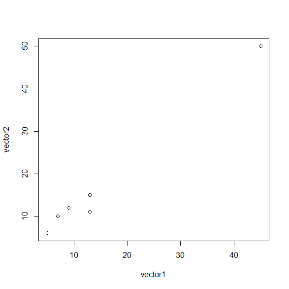
EX 1.7 So far, so good. R can also plot any two vectors (with the same length) on a 2-d plot. R can do some crazy plotting stuff but let's start with the classics. Try
plot (vector1, heartrate)
. Not bad right? Your plot should look something like this:

We'll make these plots prettier later. If you wanted to draw a line connecting these points, you could type
lines (vector1, heartrate)
to add this line to your plot. Try it. Your plot with lines added should look something like this.

EX 1.8 Positional vs. named arguments - and R expression like "plot" has things you tell it to work on or arguments. We weren't surprised that R put the first variable we listed as an argument, vector1, on the x-axis and the second on the y, because that's conventional. This is positional matching and R uses it a lot. Because sometimes there are a lot more than two arguments, we can also explicitly specify arguments like this
plot (x=vector1, y=heartrate)
, which would be the same if we flipped it
plot (y=heartrate, x=vector1)
. Try both of these. These two methods of argument can be mixed.
[ASIDE 1: If you want to repeat a command, just hit the up arrow, or ctrl-p. This is often useful to repeat a slight variation on a long command: just hit up, and edit the bit that's changed.]
[ASIDE 2: If you lose your plot window, in Windows, look for it in the "Windows” tab at the top of the R window and check it.]
EX 1.9 We can fill a vector with the sequence 9,10,11,12,13,14,15 by just typing
vector2 <- seq (9,15)
or by typing
vector2 <- 9:15
. You can also specify a spacing other than 1, e.g.
vector2 <- seq (0,20, by=2)
would put [0,2,4,6,8,10,12,14,16,18,20] into vector2. You can have an interval evenly subdivided like this:
vector2 <- seq (0,9,length = 6)
to get [0,1.5,3,4.5,6,7.5,9] . Try these.
EX 1.10 We can repeat anything n times by rep (thing, n) . Concretely,
repvector <- rep (23,10)
will fill repvector with [23,23,23,23,23,23,23,23,23,23] . If you’ve been following along, then
repvector <- rep (vector2,2)
will fill repvector with [0,1.5,3,4.5,6,7.5,9,0,1.5,3,4.5,6,7.5,9] .
NOTE: It’s easy to do some considerably more complex things with the rep expression. We will hold off checking these out until / unless they are needed for this course.
SELF-TEST 1. Try to figure out what output these commands will generate. Write your answer in, then type the command into R and see what happens.
Q1.1 seq (1,12, length = 6)
Q1.2 seq (0,12, length = 6)
Q1.3 rep (1:10,10)
Q1.4 length (rep (1:10,10))
Q1.5 mean (1:10)
Q1.6 mean (0:10)
Stretch for a second, then on to part 2. Let’s Panic About R Part II: Getting into real data sets
Ok, we’re up and running in R. Let’s start learning how to mess up some real data.
R’s idiom for importing data is the DATA FRAME. To R, a data frame is a bunch of vectors that share and index. What’s an index you ask? Let’s go over it briefly.
Indexing in R vectors.
Let’s enter a new vector for this example:
vector1 <- c(5,7,9,13,45,13)
. If we want to refer to the third element in this vector, we can say
vector1[3]
, which should give 9. Try it now.
EX 1.11 For these three, guess what they will do and then try them.
vector1[c(3,5,6)]
vector1[7]
vector1[-4]
These results should show you two new things: first, that asking for a vector element that doesn’t exist gives back a special value that R uses called “NA”, and second, that –n excludes element n when used in an index.
Now, we can return to DATA FRAMES knowing what an index is.
If we enter a second vector with the same number of elements,
vector2 <- c(6,10,12,15,50,11)
, we can now create a data frame from these two vectors. If you think of this like an Excel spreadsheet, we’re assuming each vector to be a column from a big table, where the rows in vectors 1 and 2 correspond. Let’s try it, to understand it better.
dframe1 <- data.frame(vector1, vector2)
Now let’s look at what’s in dframe1 !
dframe1
should output
vector1 vector2
1 5 6
2 7 10
3 9 12
4 13 15
5 45 50
6 13 11
, and
plot(dframe1)
should spit out something about like this:
.
Try these!
2-d indexing of a data frame matrix.
We can access a specific element in our new data frame.
EX 1.12
What do you expect from the command
dframe1[4,2]
? Try it.
This gives back 15, the value in the 4th row, 2nd column of the data frame.
Let’s make a new data frame with more descriptive columns. These are height and weight of heavyweight fighters in inches and pounds respectively.
height <- c(72, 74, 75, 68, 70, 77)
weight <- c(205, 225, 230, 225, 205, 235)
heavyweights <- data.frame(height, weight)
'Conditional selection, 'subset, and transform.
We can ask for the heights, of only those fighters whose weight is over 210 pounds, like this:
'EX 1.13' Conditional selection. Try this yourself:
height [weight > 210]
. This is called conditional selection, in R.
We can also operate on the entire data frame in a similar way, by creating a subset of the data frame.
'EX 1.14' Subsets. What would you expect for the output of these commands? Guess first, then type (don’t copy paste!) and see what happens.
subset (heavyweights, weight > 210)
subset (heavyweights, (height > 72 & weight < 235))
In the same way that we used & above to mean that both conditions must be true, we can use | to mean “or”, so either condition must be true, and ! to mean not, so the opposite.
'EX 1.15' Subsets and new operators. Guess, and try,
subset (heavyweights, (height > 72 | weight < 235))
subset (heavyweights, (height > 72 | !(weight < 235)))
Say we now want to calculate the BMI (body mass index) for all of our heavyweights, and add it to our data frame as an additional column. That’s what transform does. Let’s do this.
bmi <- transform (heavyweights, bmi = 703*(weight/height^2))
bmi
Your output should look like this:
height weight bmi
1 72 205 27.79996
2 74 225 28.88514
3 75 230 28.74489
4 68 225 34.20740
5 70 205 29.41122
6 77 235 27.86389
.
What will happen if we ask R to put your 3-d transformed data into a 2-d default plot? Only one way to find out!
'EX 1.16' Do this thing right here:
plot (bmi)
. How’s your mind – blown? Your output should look about like this:
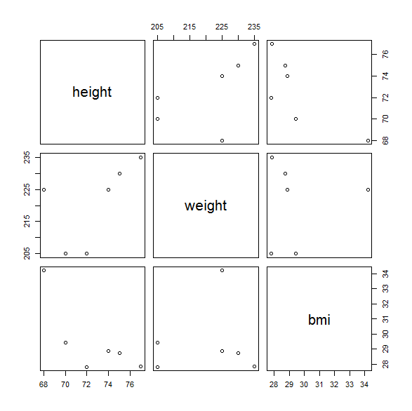
What’s going on here? This is a symmetrical double set of the 2-d plot for height vs weight, height vs bmi, and weight vs bmi, respectively. When you ask R to do something, it likes to make some default assumptions and take the ball and run with it, rather than prompting you for more specifics, if it can help it. Thanks, R.
Implicit loops
What if we want to do the same thing, to every column in a data frame, like get the mean of each column, or the variance? We can use implicit loops- they just loop over each column automatically.
lapply(bmi, mean)
will just run the mean expression on each column I turn.
EX 1.17 Try this, for mean, standard deviation (sd), and median. Then try using sapply instead of lapply. See the difference?
read.table
You might think that typing in a series of vectors is not the way you’d usually want to get some data into R. Good thinking. R has commands for importing data, the prototype one is read.table which reads whitespace-delimited text files, but there are also read.csv , read.csv2 , read.delim and read.delim2, which read comma separated variables, comma separated variables when the comma is also used as the decimal point (European style), tab delimited text files, etc. We’ll try a couple of these now.
In order to read in a file, we need a file to read in. You ideally want to make these files in a text editor not a word processor. gedit, vim, emacs, notepad, that kind of thing.
Let’s make a new text file that looks like this:
Name Status
Kaeberlein Director
McCormick TA
Lee TA
Promislow Director
Leiser TA
Miller TA
Here the words on the same line are separated by a space, and the lines are separated by the ENTER key (a newline character). Type this into a file and save it as lecture1-textfile1.txt . You’ll need to know where this file is saved to in your directory, e.g. if it were in C:/Users/mark/Documents/ etc. We will probably sort out where it is saving to by default on the course MacBooks live in class. Help your neighbor.
EX 1.18 Then try your equivalent of
read.table("C:/Users/mark/Documents/lecture1-textfile1.txt",header=T)
depending on your file’s path. What happens if you try the same command with header=F ? Try it.
Notice that this data is not numbers, it’s all text. We can consider the text to be a description of categories, in particular the second column divides errbody into two groups. R can sort these, check it:
EX 1.19
staff <- read.table("C:/Users/mark/Documents/lecture1-textfile1.txt",header=T)
names.ta <- staff$Name[staff$Status==’TA’]
names.ta
EX 1.20 Now make a new thing, names.director, you know the rest!
Let’s get self-sufficient.
R has a lot of built-in help. If you wanted to ask R how to do something with read.table, you could just use ?read.table . Note the question mark. You can figure out a ton by yourself in a pinch using this method. Baby steps. apropos() is like Google suggest for the ? command: it just searches for anything that’s a text match to whatever is in the () – good if you know what you want to do but aren’t positive you know the exact spelling of the R expression. Actual Google searches are a bomb way to uncover how to do something in R as well.
EX 1.21 Check the help for read.table, and the help for write.table. Using what you learn, save your staff data frame as a comma-separated-variable (csv) file, then read it back in from the csvfile as staffcsv, a new data frame. Display it to be sure that it has worked correctly.
As an ASIDE: Microsoft Excel, and the completely free and open source LibreOffice, among many others, offer the option of saving data into csv and tab-delimited text files, which allows easy import from spreadsheet data into R.
EX 1.22 What will happen if you try plot(staff) ? Do this. R will always take a shot at it with some default assumptions. If you want it to do something different than its default behavior you can customize the output; more on that soon.
….
Ok, this is soon enough. More on plots!
Titles and subtitles
EX 1.23 Using ?title and ?plot, figure out how to replot the plot(staff) but with a title above the graph that says “EX 1.23”, and the x-axis label changed from Name to Last Name.
par
par does a ton of stuff. You can control all of the fonts, sizes and spacing, and colors in a plot through par. It’s easiest to learn par by playing around with different options one or two at a time, especially since the default plot parameters are usually nice choices.
EX 1.24 Using the appropriate ? command, sort out how to re-plot staff but with a red background.
Combining plots, and a hint of things in the next lecture
Let’s overlay or combine two plots in one plot window, in just a second. First, to get something fun to overlay, we’ll learn a couple of new commands. First is rnorm
rnorm
rnorm(n)generates n random variates of a standard normal distribution (mean 0 sd 1), and is useful for simulating normally distributed experimental data, among other things. We will learn more about it in a sec, and even more later on. set.seed and generating reproducible data with R random functions. R uses a pseudo-random number generator to do things like rnorm. Each time you use rnorm(100), you will get a slightly different result, because there is a different seed for pseudo-random number generation. If you want to specify a particular seed, you use set.seed(somenumber) . This way, if you need to turn in a homework result, or ask a colleague or internet message board for help with something, you can make sure the other person gets exactly the same “random” data as you by setting the same seed.
hist
hist draws a histogram. Again, we will start simple and learn more about the advanced options of hist later on; you can always skip ahead using ? .
curve
curve draws a curve corresponding to a function that you give it. Again, more later and use ? !!
Okay now. Let’s make some random data, plot it as a histogram, and overlay the normal distribution of the data.
EX 1.25 Let’s make 100 random deviates from a standard normal distribution
x<-rnorm(100)
Now let’s plot a histogram of x by frequency. We will talk a bit now about what this means, and a lot more about it on Friday.
hist(x,freq=F)
Now let’s overlay the actual normal distribution we just showed the histogram of
curve(dnorm(x),add=T)
Sweet. Now: EX 1.26 Now, repeat all of the commands above three or four times. Your curve will stay the same, but your histogram will vary because rnorm is pseudo-random. Then, set your seed to 100 and try it again- you should get the same histogram as your neighbor if they’ve set their seed to 100. Our default set.seed for the class will be 100 btw.
The workspace
Your R session has a workspace. This is just a record of what’s stored in what variables, and what packages are loaded, etc. you can save all the details of an open workspace to a file any time with
save.image()
and R will ask if you want to load the saved workspace when you start it.
You can see what’s in your workspace with
ls()
and delete anything from your current ls list with
rm(thingyouwanttodelete)
.
Packages, data sets, and the data editor
Packages are extra bits of software that add even more capability to R, and there are a TON of them. You can find many at http://cran.us.r-project.org/ . To install a new package, check back to our very first commands in this lecture. To then use a package, use the command library(packagename) which loads the package for use in the current R session or script.
EX 1.27 Install and load the survival package.
You can attach data sets in R with the attach command, and get rid of them with the detach command. There are a lot of example data sets that R will load by default, and public data sets that can be attached by specifying where they are.
EX 1.28 Attach and then detach the trees and iris data sets, and display them.
R has a built-in spreadsheet like data viewer and editor that is ok for quick simple edits.
EX 1.29 Use ? as needed– attach iris and plot it. Assign an edited version of iris to editediris, in which the first two virginica cells are changed to sasquathica. Now plot editediris.
HOMEWORK
For this, submit an R file, and save any plots as images, and any exported txt or csv as directed- just zip it all up into a zip file for lecture 1. Work together and help each other, but if you can’t do each one on your own you’ll be hosed by the end of the following lecture.
1. Create a ‘.csv’ formatted dataset in Excel with the following data Month Year AvgTemp Jan 2008 50 Jan 2009 46 Jan 2010 39 April 2008 58 April 2009 63 April 2010 59 July 2008 85 July 2009 78 July 2010 95 Sept 2008 69 Sept 2009 65 Sept 2010 67
Import these data into R (use the ‘Change working directory’ command under the “Misc” menu to (you guessed it!) change the working directory, specifying where R can find the file that you created. Create a boxplot of AvgTemp as a function of Month Calculate the average temperature by month, and save the data back onto your computer.
2. Attach the iris dataset. Create three new objects that contain only the versicolor, setosa, and virginica rows of the dataset. Plot sepal.length vs. sepal.width for each of these subsets on the same plot, with each displayed in a different color. Repeat for petal.length vs. petal.width.